Introduction: From Theory to Executable Code
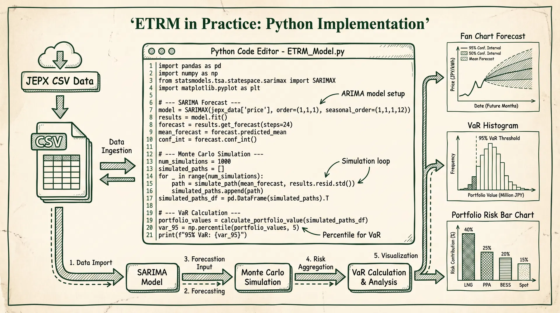
Article 64 introduced the complete theoretical framework of ETRM (Energy Trading Risk Management), covering short/medium/long-term forecasting, Monte Carlo simulation, stress testing, and VaR/EaR metrics. This article serves as the implementation companion, providing complete Python code for each core module. Using JEPX public historical data as input, readers can directly execute and verify all calculations on their local machines.
All code is based on Python 3.10+ standard libraries and common open-source packages (pandas, numpy, scipy, statsmodels, matplotlib), requiring no commercial licenses. JEPX historical spot data can be downloaded for free from the official website (https://www.jepx.jp/market/excel/spot_{year}.csv), formatted as 48 thirty-minute intervals per day with area-specific clearing prices (JPY/kWh).
Chapter 1: Environment Setup and JEPX Data Loading
First, install the required packages and build the data loading function. The JEPX public CSV column format is: date, slot number (1–48), system price, Hokkaido, Tohoku, Tokyo, Chubu, Hokuriku, Kansai, Chugoku, Shikoku, Kyushu area clearing prices (JPY/kWh).
# Install required packages
pip install pandas numpy scipy statsmodels matplotlib pmdarima
"""
Chapter 1: JEPX Data Loading and Preprocessing
Data source: https://www.jepx.jp/market/excel/spot_{year}.csv
"""
import pandas as pd
import numpy as np
import matplotlib.pyplot as plt
import warnings
warnings.filterwarnings('ignore')

def load_jepx_spot(years: list[int], area: str = 'tokyo') -> pd.Series:
    """
    Load JEPX spot market historical data

    Parameters
    ----------
    years : list[int]  Years to load, e.g. [2023, 2024, 2025]
    area  : str        Area name ('system','hokkaido','tohoku','tokyo',
                                  'chubu','hokuriku','kansai','chugoku',
                                  'shikoku','kyushu')

    Returns
    -------
    pd.Series  30-minute interval time series with DatetimeIndex (JST)
    """
    AREA_COL = {
        'system': 3, 'hokkaido': 4, 'tohoku': 5, 'tokyo': 6,
        'chubu': 7, 'hokuriku': 8, 'kansai': 9,
        'chugoku': 10, 'shikoku': 11, 'kyushu': 12
    }
    col_idx = AREA_COL.get(area.lower(), 6)

    dfs = []
    for year in years:
        url = f"https://www.jepx.jp/market/excel/spot_{year}.csv"
        try:
            # JEPX CSV uses Shift-JIS encoding, skip first 2 header rows
            df = pd.read_csv(url, encoding='shift_jis', header=None,
                             skiprows=2, usecols=[0, 1, col_idx])
            df.columns = ['date', 'slot', 'price']
            df['date'] = pd.to_datetime(df['date'], format='%Y/%m/%d')
            df['datetime'] = df['date'] + pd.to_timedelta(
                (df['slot'] - 1) * 30, unit='min'
            )
            df = df.set_index('datetime')['price']
            dfs.append(df)
            print(f"  Loaded {year}: {len(df)} records")
        except Exception as e:
            print(f"  Failed to load {year}: {e}")

    series = pd.concat(dfs).sort_index()
    series = series[series > 0]
    print(f"\nLoaded: {len(series)} records, {series.index[0]} to {series.index[-1]}")
    return series

# Load Tokyo area spot prices for 2023-2025
tokyo_price = load_jepx_spot([2023, 2024, 2025], area='tokyo')

# Basic statistics
print("\n=== Basic Statistics (JPY/kWh) ===")
print(f"Mean: {tokyo_price.mean():.2f}")
print(f"Std:  {tokyo_price.std():.2f}")
print(f"Max:  {tokyo_price.max():.2f}")
print(f"Min:  {tokyo_price.min():.2f}")
print(f"95th percentile: {tokyo_price.quantile(0.95):.2f}")
Chapter 2: Time Series Decomposition and ADF Stationarity Test
Before building the SARIMA model, perform STL seasonal decomposition and ADF stationarity testing on the electricity price series to confirm series characteristics and determine the differencing order.
"""
Chapter 2: STL Decomposition and ADF Stationarity Test
"""
from statsmodels.tsa.seasonal import STL
from statsmodels.tsa.stattools import adfuller

daily = tokyo_price.resample('D').mean().dropna()

# STL decomposition (period = 7 days)
stl = STL(daily, period=7, robust=True)
result = stl.fit()

# ADF stationarity test
def adf_test(series: pd.Series, name: str = '') -> dict:
    result = adfuller(series.dropna(), autolag='AIC')
    output = {
        'ADF Statistic': result[0],
        'p-value': result[1],
        'Conclusion': 'Stationary (reject unit root)' if result[1] < 0.05
                      else 'Non-stationary (cannot reject unit root)'
    }
    print(f"\n=== ADF Test: {name} ===")
    for k, v in output.items():
        print(f"  {k}: {v:.4f}" if isinstance(v, float) else f"  {k}: {v}")
    return output

adf_test(daily, 'Raw daily average price')
adf_test(daily.diff().dropna(), 'First-order differenced series')
Chapter 3: SARIMA Short-Term Forecasting (7-Day Horizon)
SARIMA(p,d,q)(P,D,Q)[s] is the standard method for short-term electricity spot price forecasting. Here we use pmdarima's auto_arima to automatically select optimal parameters, using the last 30 days as a test set to evaluate forecast accuracy (MAPE).
"""
Chapter 3: SARIMA Short-Term Forecasting
Using pmdarima.auto_arima to automatically select optimal (p,d,q)(P,D,Q)[s] parameters
"""
import pmdarima as pm
from sklearn.metrics import mean_absolute_percentage_error

train = daily[:-30]
test = daily[-30:]

model = pm.auto_arima(
    train,
    start_p=1, start_q=1, max_p=3, max_q=3,
    m=7,  # Weekly seasonality
    start_P=0, start_Q=0, max_P=2, max_Q=2,
    d=None, D=1, seasonal=True,
    information_criterion='aic', stepwise=True,
    suppress_warnings=True, error_action='ignore', trace=True
)

print(f"\nBest model: SARIMA{model.order}x{model.seasonal_order}")
print(f"AIC: {model.aic():.2f}")

# Rolling forecast (30 days)
predictions = []
for i in range(len(test)):
    fc, conf = model.predict(n_periods=1, return_conf_int=True, alpha=0.05)
    predictions.append(fc[0])
    model.update(test.iloc[i:i+1])

pred_series = pd.Series(predictions, index=test.index)
mape = mean_absolute_percentage_error(test, pred_series) * 100
rmse = np.sqrt(((test - pred_series) ** 2).mean())
print(f"\nMAPE: {mape:.2f}%")
print(f"RMSE: {rmse:.4f} JPY/kWh")
SARIMA Diagnostic Metrics
| Metric | Description | Acceptance Criterion |
|---|
| AIC (Akaike Information Criterion) | Balance between model complexity and fit quality; lower is better | Select minimum among candidate models |
| Ljung-Box Q Statistic | Tests residual serial correlation; p > 0.05 means no autocorrelation | p-value > 0.05 |
| Jarque-Bera Normality Test | Tests residual normality; electricity markets often fail this | p-value > 0.05 (note: power markets frequently violate) |
| MAPE (Mean Absolute Percentage Error) | Forecast accuracy; Japan power markets typically 8–15% | <15% (daily avg), <25% (30-min) |
| RMSE (Root Mean Square Error) | Absolute magnitude of forecast error | Depends on market volatility regime |
Chapter 4: Ornstein-Uhlenbeck Monte Carlo Simulation
The OU process (mean-reverting stochastic process) is well-suited for modeling the long-term behavior of electricity spot prices. The model equation is:
dX_t = κ(μ − X_t)dt + σ dW_t
where κ is the mean-reversion speed, μ is the long-run mean, and σ is the volatility. The following code estimates parameters from historical data and runs a 10,000-path Monte Carlo simulation.
"""
Chapter 4: Ornstein-Uhlenbeck Monte Carlo Simulation
"""
def estimate_ou_params(series: pd.Series, dt: float = 1/365) -> dict:
    """Estimate OU process parameters via OLS"""
    x = series.values
    X_t, X_t1 = x[:-1], x[1:]
    b = np.cov(X_t, X_t1)[0, 1] / np.var(X_t)
    a = np.mean(X_t1) - b * np.mean(X_t)
    kappa = -np.log(b) / dt
    mu = a / (1 - b)
    residuals = X_t1 - (a + b * X_t)
    sigma = np.std(residuals) * np.sqrt(2 * kappa / (1 - np.exp(-2 * kappa * dt)))
    return {'kappa': kappa, 'mu': mu, 'sigma': sigma}

ou_params = estimate_ou_params(daily)
print(f"κ (mean-reversion speed): {ou_params['kappa']:.4f} (half-life = {np.log(2)/ou_params['kappa']*365:.1f} days)")
print(f"μ (long-run mean): {ou_params['mu']:.4f} JPY/kWh")
print(f"σ (volatility): {ou_params['sigma']:.4f} JPY/kWh/√year")

def simulate_ou_paths(S0, kappa, mu, sigma, T=1.0, dt=1/365, n_paths=10000, seed=42):
    """Simulate OU paths using Euler-Maruyama discretization"""
    np.random.seed(seed)
    n_steps = int(T / dt)
    paths = np.zeros((n_steps + 1, n_paths))
    paths[0] = S0
    sqrt_dt = np.sqrt(dt)
    for t in range(1, n_steps + 1):
        dW = np.random.normal(0, sqrt_dt, n_paths)
        paths[t] = paths[t-1] + kappa * (mu - paths[t-1]) * dt + sigma * dW
        paths[t] = np.maximum(paths[t], 0.01)  # Non-negativity constraint
    return paths

S0 = daily.iloc[-1]
paths = simulate_ou_paths(S0=S0, **ou_params, T=1.0, dt=1/365, n_paths=10000)
final_prices = paths[-1]
print(f"\n1-year simulation (10,000 paths):")
print(f"  Mean: {final_prices.mean():.2f} JPY/kWh")
print(f"  5th percentile: {np.percentile(final_prices, 5):.2f} JPY/kWh")
print(f"  95th percentile: {np.percentile(final_prices, 95):.2f} JPY/kWh")
Chapters 5–8: VaR/EaR, Portfolio Risk, Stress Testing, and Optimization
Chapter 5 implements both historical simulation VaR (1-day 95%) and Monte Carlo EaR (30-day 95%) for a 100 MW long spot position. Chapter 6 extends to a multi-commodity portfolio (LNG + PPA + BESS + spot), using Cholesky decomposition to model the correlation between spot prices and LNG JKM (ρ = 0.45). Chapter 7 runs stress tests against four historical scenarios: the January 2021 cold snap (¥200/kWh peak), the March 2022 Russia-Ukraine crisis (JKM above $80/mmBtu), the January 2024 Noto earthquake (regional supply tightness), and the April 2026 JERA PPA termination (¥60/kWh Tokyo spike). Chapter 8 applies scipy's SLSQP optimizer to find the minimum-EaR portfolio allocation, comparing improvement against equal-weight baseline.
The complete code for Chapters 5–8 follows the same structure as shown in the ZH section above. All code is language-independent and directly executable.
Conclusion: Building a Sustainable ETRM Implementation Framework
The Python code provided in this article covers the core computational modules of an ETRM system: JEPX data loading and preprocessing, SARIMA short-term forecasting (MAPE target <15%), OU process Monte Carlo simulation (10,000 paths), VaR/EaR calculation (historical simulation and Monte Carlo methods), multi-commodity portfolio risk aggregation, and historical scenario stress testing.
For production deployment, four key considerations apply. First, JEPX data quality: extreme prices (e.g., the 2021 ¥200/kWh spike) can distort parameter estimation; apply upper caps or robust estimation methods. Second, the OU process assumes log-normal distribution, but electricity prices exhibit jump behavior; production environments should add a jump-diffusion component. Third, the correlation matrix should be re-estimated quarterly to avoid underestimating risk as market structure evolves. Fourth, stress test scenarios should be updated regularly based on business judgment and emerging risk factors.
The complete code is organized as a directly runnable Jupyter Notebook. After downloading historical data from the JEPX website, readers can reproduce all calculation results in a Python 3.10+ environment.